
贝叶斯线性回归(Bayesian linear regression)是使用统计学中贝叶斯推断(Bayesian inference)方法求解的线性回归(linear regression)模型。
贝叶斯线性回归将线性模型的参数视为随机变数(random variable),并通过模型参数(权重係数)的先验(prior)计算其后验(posterior)。贝叶斯线性回归可以使用数值方法求解,在一定条件下,也可得到解析型式的后验或其有关统计量。
贝叶斯线性回归具有贝叶斯统计模型的基本性质,可以求解权重係数的机率密度函式,进行线上学习以及基于贝叶斯因子(Bayes factor)的模型假设检验。
基本介绍
- 中文名:贝叶斯线性回归
- 外文名:Bayesian linear regression
- 类型:回归算法
- 提出者:Dennis Lindley,Adrian Smith
- 提出时间:1972年
- 学科:统计学
历史
贝叶斯线性回归是二十世纪60-70年代贝叶斯理论兴起时得到发展的统计方法之一,其早期工作包括在回归模型中对权重先验和最大后验密度(Highest Posterior Density, HPD)的研究、在贝叶斯视角下发展的随机效应模型(random effect mode)以及贝叶斯统计中可交换性(exchangeability)概念的引入。
正式提出贝叶斯回归方法的工作来自英国统计学家Dennis Lindley和Adrian Smith,在其1972年发表的两篇论文中,Lindley和Smith对贝叶斯线性回归进行了系统论述并通过数值试验与其它线性回归方法进行了比较,为贝叶斯线性回归的套用奠定了基础。
理论与算法
模型
给定相互独立的N组学习样本 ,
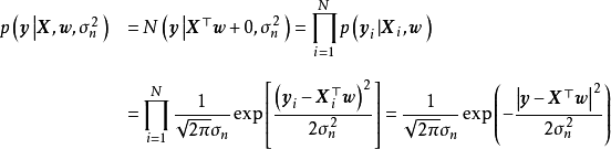
, ,贝叶斯线性回归使用如下的多元线性回归模型
 :
:


求解
根据线性模型的定义,权重係数 与观测数据
与观测数据 相互独立,也与残差的方差
 相互独立,由贝叶斯定理(Bayes' theorem)可推出,贝叶斯线性回归中权重係数的后验有如下表示:


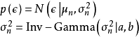
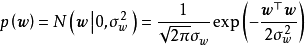
求解 式要求预先给定权重係数的先验 ,即一个连续机率分布(continuous probability distribution),通常的选择为0均值的常态分配:

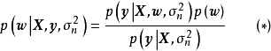
先验、似然和后验,(b)回归结果") 一维贝叶斯线性回归:(a,c,d)先验、似然和后验,(b)回归结果
一维贝叶斯线性回归:(a,c,d)先验、似然和后验,(b)回归结果在权重係数没有合理先验假设的问题中,贝叶斯线性回归可使用无信息先验(uninformative prior),即一个均匀分布(uniform distribution),此时权重係数按均等的机会取任意值。
极大后验估计(Maximum A Posteriori estimation, MAP)
在贝叶斯线性回归中,MAP可以被视为一种特殊的贝叶斯估计(Bayesian estimator),其求解步骤与极大似然估计(maximum likelihood estimation)类似。对给定的先验,MAP将 式转化为求解 使后验机率最大的最佳化问题,并求得后验的众数(mode)。由于常态分配的众数即是均值,因此MAP通常被套用于正态先验。
这里以的0均值正态先验为例介绍MAP的求解步骤,首先给定权重係数 的0均值常态分配先验:
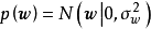 。由于边缘似然与
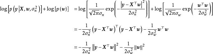
 相互独立,此时求解后验机率的极大值等价于求解似然和先验乘积的极大值:


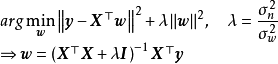


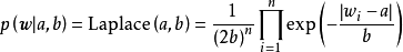
除正态先验外,MAP也使用拉普拉斯分布(Laplace distribution)作为权重係数的先验:


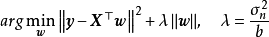

MAP是单点估计,不支持线上学习(online learning),也无法提供置信区间,但能够以很小的计算量求解贝叶斯线性回归的权重係数,且可用于最常见的正态先验情形。使用正态先验和MAP求解的贝叶斯线性回归等价于岭回归(ridge regression),最佳化目标中的 被称为L2正则化项;使用拉普拉斯分布先验的情形对应线性模型的LASSO(Least Absolute Shrinkage and Selection Operator),
 被称为L1正则化项。
共轭先验求解
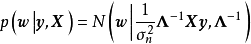
由于贝叶斯线性回归的似然是常态分配,因此在权重係数的先验存在共轭分布时可利用共轭性(conjugacy)求解后验。这里以正态先验为例介绍其求解步骤。
首先引入权重係数的0均值正态先验: ,随后由 式可知,后验正比于似然和先验的乘积:


除正态先验外,共轭先验求解也适用于对数常态分配(log-normal distribution)、Beta分布(Beta distribution)、Gamma分布(Gamma distribution)等的先验。
数值方法
一般地,贝叶斯推断的数值方法都适用于贝叶斯线性回归,其中最常见的是马尔可夫链蒙特卡罗(Markov Chain Monte Carlo, MCMC)。这里以MCMC中的吉布斯採样(Gibbs sampling)算法为例介绍。
给定均值为 ,方差为
,方差为 的正态先验
的正态先验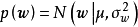 和权重係数
和权重係数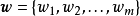 ,吉布斯採样是一个叠代算法,每个叠代都依次採样所有的权重係数:
1. 随机初始化权重係数 和残差的方差
2. 採样 :
:
3. 使用 採样 :
:
4. 採样 :
:
5. 重複1-4至叠代完成/分布收敛
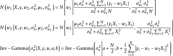
叠代步骤中的 和
和 被称为条件採样分布(conditional sampling distribution)。条件採样的推导较为繁琐,这里给出一维情形下截距
 、斜率
、斜率 和残差方差
和残差方差 的条件採样分布:
在Python 3的Numpy模组下,上述叠代步骤可有如下编程实现:
import numpy as npimport matplotlib.pyplot as plt# 构建测试数据## 自变数:[0,5]区间均匀分布x = np.random.uniform(low=0, high=5, size=5)## 因变数:y=2x-1+eps, eps=norm(0, 0.5)y = np.random.normal(2*x-1, 0.5)def calculate_csd(x, y, w1, w2, s, N, hyper_param): ''' 条件採样分布函式: (w1, w2, s) x , y: 输入数据 w1, w2: 线性回归模型的截距和斜率 s: 残差方差 N: 样本量 ''' # 超参数 mu1, s1 = hyper_param["mu1"], hyper_param['s1'] mu2, s2 = hyper_param["mu2"], hyper_param['s2'] a, b, = hyper_param["a"], hyper_param["b"] # 计算方差 var1 = (s1*s)/(s+s1*N) var2 = (s*s2)/(s+s2*np.sum(x*x)) # 计算均值 mean1 = (s*mu1+s1*np.sum(y-w2*x))/(s+s1*N) mean2 = (s*mu2+s2*np.sum((y-w1)*x))/(s+s2*np.sum(x*x)) # 计算(a, b) eps = y-w1-w2*x a = a+N/2; b = b+np.sum(eps*eps)/2 # 使用numpy.random採样(inv-gamma=1/gamma) # 注意numpy.random中normal和gamma的定义方式: ## np.random.normal(mean, std) ## inv-Gamma = 1/np.random.gamma(a, scale), scale=1/b return np.random.normal(mean1, np.sqrt(var1)), np.random.normal(mean2, np.sqrt(var2)), 1/np.random.gamma(a, 1/b)def Gibbs_sampling(x, y, iters, init, hyper_param): ''' 吉布斯採样算法主程式 iter: 叠代次数 init: 初始值 hyper_param: 超参数 ''' N = len(y) # 样本量 # 採样初始值 w1, w2, s = init["w1"], init["w2"], init["s"] # 使用数组记录叠代值 history = np.zeros([iters, 3])*np.nan # for循环叠代 for i in range(iters): w1, w2, s = calculate_csd(x, y, w1, w2, s, N, hyper_param) history[i, :] = np.array([w1, w2, s]) return history# 开始採样iters = 10000 # MCMC叠代1e4次init = {'w1': 0, 'w2': 0, 's': 0}hyper_param = {'mu1': 0, 's1': 1, 'mu2': 0, 's2': 1, 'a': 2, 'b': 1}history = Gibbs_sampling(x, y, iters, init, hyper_param)burnt = history[500:] # 截取收敛后的马尔可夫链ax1 = plt.subplot(2, 1, 1); ax2 = plt.subplot(2, 1, 2)ax1.hist(burnt[:, 0], bins=100)ax1.text(2, 0.025*iters, '$mathrm{N(w_1|mu,s)}$', fontsize=14)ax2.hist(burnt[:, 1], bins=100)ax2.text(.5, 0.025*iters, '$mathrm{N(w_2|mu,s)}$', fontsize=14)除吉布斯採样外,Metropolis-Hastings算法和数据增强算法(data augmentation algorithm)也可用于贝叶斯线性回归的MCMC计算。
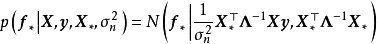
预测
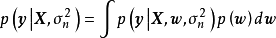
由MAP求解的贝叶斯线性回归可直接使用权重係数对预测数据进行计算。MAP是单点估计,因此预测结果不提供后验分布。对共轭先验或数值方法求解的贝叶斯线性回归,可通过边缘化(marginalized out)模型权重,即按其后验积分得到预测结果:


模型验证
边缘似然描述了似然和先验的组合在多大程度上解释了观测数据,因此边缘似然可以用于计算贝叶斯因子,与其它模型进行比较并验证模型和先验的合理性。由全机率公式(law of total probability)可知,边缘似然有如下积分形式:
由MCMC计算的贝叶斯线性回归也可以使用数值方法进行交叉验证(cross-validation),具体方法包括重採样(re-sampling MCMC)和使用EC(Expectation Consistent)近似的留一法(Leave One Out, LOO)交叉验证。
线上学习
由共轭先验和数值方法求解的贝叶斯线性回归可以进行线上学习,即使用实时数据对权重係数进行更新。线上学习的具体方法依模型本身而定,其设计思路是将先钱求解得到的后验作为新的先验,并带入数据得到后验。
性质
稳健性:由求解部分的推导可知,若贝叶斯线性回归使用正态先验,则其MAP的估计结果等价于岭回归,而使用拉普拉斯先验的情形对应线性模型的LASSO,因此贝叶斯线性回归与使用正则化(regularization)的回归分析一样平衡了模型的经验风险和结构风险。特别地,使用拉普拉斯先验的贝叶斯线性回归由于可以得到稀疏解,因此具有一定的变数筛选(variable selection)能力。
作为贝叶斯推断所具有的性质:由于贝叶斯线性回归是贝叶斯推断线上性回归问题中的套用,因此其具有贝叶斯方法的一般性质,包括对先验进行实时更新、将观测数据视为定点因而不需要渐进假设、服从似然定理(likelihood principle)、估计结果包含置信区间等。基于最小二乘法的线性回归(Ordinary Linear Regression, OLR)通常仅在观测数据显着地多于权重係数维数的时候才会有好的效果,而贝叶斯线性回归没有此类限制,且在权重係数维数过高是,可以根据后验对模型进行降维(dimensionality reduction)。
与高斯过程回归(Gaussian Process Regression, GPR)的比较:贝叶斯线性回归是GPR在权重空间(weight-space)下的特例。在贝叶斯线性回归中引入映射函式 可得到GPR的预测形式:
 ,而当映射函式为等值函式(identity function)时,GPR退化为贝叶斯线性回归。
套用
除一般意义上线性回归模型的套用外,贝叶斯线性模型可被用于观测数据较少但要求提供后验分布的问题,例如对物理常数的精确估计。有研究利用贝叶斯线性回归的性质进行变数筛选和降维。此外,贝叶斯线性回归是在统计方法中使用贝叶斯推断的简单实现之一,因此常作为贝叶斯理论或数值计算教学的重要例子。


